2021 Third report complement: Comparison of Sea Ice Forecasts Using Simple Regression and Multiple Regression Analysis
In the first and second reports, prediction calculations were made by the correlation between the density of particles on sea ice and the sea ice concentration. In the third report, we added sea ice age, a new variable to perform a multiple regression analysis for prediction calculation. We explain the method and the differences from the results of the previous method.
Multiple regression analysis
In the first and second reports, we determined the correlation between the density of particles on the sea ice at the end of April and May (reflecting the change in sea ice thickness from the previous winter to spring) and the deviation from the linear trend of sea ice concentration by simple regression analysis and used it for forecasting. In the third report, we added the sea ice age to perform multiple regression analysis for prediction calculation. In general, the older the sea ice is thicker, sea ice age is considered to reflect long-term changes in sea ice thickness compared to particle density. By adding the information of sea ice age to the prediction, the distribution of thick ice that has grown over many years are considered. In this analysis, the multiple regression equation is calculated as follows.
\begin{align*}
(SIC’)^{n}_{i,j} = a \cdot{} P^{n}_{i,j} + b \cdot{} (SIA)^{n}_{i,j} + c \tag{1}
\end{align*}
Let Equation$(1)$ be the multiple regression equation to obtain. Here, $SIC’$ is the deviation of sea ice concentration from the linear trend obtained by the regression plane, $P$ is the density of particles, $SIA$ is the sea ice age, $n$ is the year, $i,j$ are the coordinates of the grid points, and $a,b,c$ are the constants that determine the regression plane, which are obtained by using the least-squares method. Since the least-squares method determines each constant so that the square sum of the deviations between the regression plane and the measured value is minimized, $a,b,c$ are found so that the partial differentiation of equation $(2)$ with each constant to be zero.
\begin{align*}
\sum_{\begin{matrix}
7 \le n \le 11 \\
16 \le n \le 20\
\end{matrix}}
(SIC’)^{n}_{i,j} = ((SIC)^n-(SIC’)^n)^2 =
\sum_{\begin{matrix}
7 \le n \le 11 \\
16 \le n \le 20\
\end{matrix}}
(a \cdot{} P^{n} + b \cdot{} (SIA)^{n} + c – (SIC’)^n)^2 \tag{2}
\end{align*}
Here, $SIC$ is the deviation from the linear trend of sea ice concentration. The subscripts $i,j$ are omitted because the position is fixed. Putting together the results of partial differentiation of equation $(2)$ with the condition that it becomes $0$ leads to 3 linear simultaneous equations as shown in equation $(3)$, which can be solved to obtain the constants $a,b,c$ that determine the regression plane.
\begin{align*}
\left\{
\begin{array}{l}
aS_{xx} + bS_{xy} + cS_{x} = S_{xz} \\
aS_{yy} + bS_{xy} + cS_{y} = S_{yz} \tag{3}\\
aS_{x} + bS_{y} + cn = S_{z} \\
\end{array}
\right.
\end{align*}
\begin{align*}
S_{x}=
\sum_{\begin{matrix}
7 \le n \le 11 \\
16 \le n \le 20\
\end{matrix}}
(P^{n}),
\qquad
S_{y}=
\sum_{\begin{matrix}
7 \le n \le 11 \\
16 \le n \le 20\
\end{matrix}}
((SIA)^{n}),
\qquad
S_{z}=
\sum_{\begin{matrix}
7 \le n \le 11 \\
16 \le n \le 20\
\end{matrix}}
((SIC’)^{n}),
\end{align*}
\begin{align*}
S_{xx}=
\sum_{\begin{matrix}
7 \le n \le 11 \\
16 \le n \le 20\
\end{matrix}}
(P^{n})^{2},
\qquad
S_{yy}=
\sum_{\begin{matrix}
7 \le n \le 11 \\
16 \le n \le 20\
\end{matrix}}
((SIA)^{n})^{2},
\end{align*}
\begin{align*}
S_{xy}=
\sum_{\begin{matrix}
7 \le n \le 11 \\
16 \le n \le 20\
\end{matrix}}
(P^{n} \cdot (SIA)^{n}),
\qquad
S_{xz}=
\sum_{\begin{matrix}
7 \le n \le 11 \\
16 \le n \le 20\
\end{matrix}}
(P^{n} \cdot (SIC’)^{n}),
\qquad
S_{yz}=
\sum_{\begin{matrix}
7 \le n \le 11 \\
16 \le n \le 20\
\end{matrix}}
((SIA)^{n} \cdot (SIC’)^{n})
\end{align*}
In this analysis, the simultaneous equations were solved with the Cramer’s rule.
The regression plane calculated above is used to obtain the deviation from this year’s linear trend, which is added to this year’s linear trend to obtain the analysis results shown in the right side of Figure 1 shown below.
Sea ice distribution

Figure 1 shows the sea ice prediction from July 1 to September 20, considering the sea ice conditions on June 30, 2021. The left figure shows the sea ice predictions obtained by the methods used in the first and second reports, and the right figure shows the sea ice predictions obtained by the method used in the third report. Comparing the two figures, we can see that there is no significant difference in the area around the Kara Sea, but the results of simple regression analysis show more sea ice loss in the area around the Laptev Sea than that of multiple regression analysis. In addition, the results from multiple regression analysis show that sea ice is more likely to remain in the Beaufort Sea. One of the possible reasons for these differences is the difference in the number of years of data used in the simple and multiple regression analysis. The sea ice age used in the multiple regression analysis is calculated over the past four years, which reduces the number of years of data available. Specifically, the simple regression analysis uses 17 years of data from 2003 to 2020, excluding 2012, while the multiple regression analysis uses 10 years of data from 2007 to 2011 and 2016 to 2020.
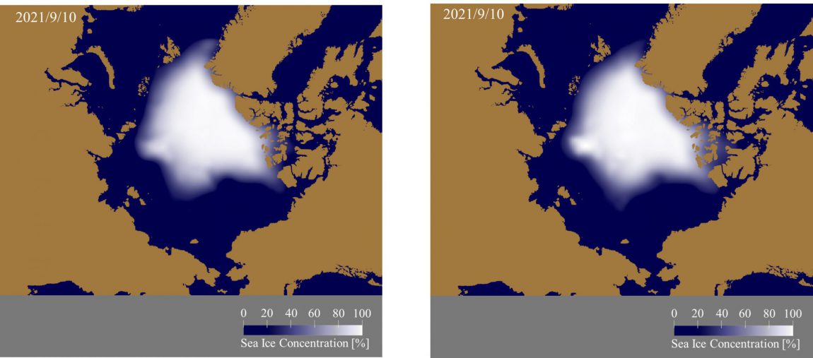
Left: Results considering 17 years of data from 2003 to 2020, excluding 2012.
Right: Results considering 10 years of data from 2007 to 2011 and from 2016 to 2020.
When the number of data used in the simple regression analysis is the same as in the multiple regression analysis (Fig. 2), the speed of sea ice loss around the Laptev Sea is close to the results of the multiple regression analysis. On the other hand, there is no significant change in the prediction around the Beaufort Sea even when the number of years of data used in the simple regression analysis is changed. This suggests that the delay in sea ice retreat in the Beaufort Sea seen in the results of the multiple regression analysis is not due to the small number of data used, but reflects the effect of old multi-year ice.